Achieving Stable Flight: The Key to Robust Control of a Quadrotor

If you want to skip the post and look at the entire report you can find the report below:

Abstract—This project addresses the need for reliable autonomous hover control systems for quadcopters, particularly in scenarios where human intervention is limited or communication is disrupted. We discuss the design of an optimal and a robust control for a Quadcopter. A linearized model about hovering conditions was extracted from a non-linear plant and was used to design a H∞ Controller. A robust controller was synthesized using the DK- iteration on MATLAB and was simulated to assess it’s robustness under parametric uncertainty in its mass and inertia. The controller offers a practical solution for autonomous hover control, bridging the gap between theoretical design and real-world implementation.

Quadrotor Dynamics:

Quadrotors have four motors in a cross configuration with two opposite rotors rotating in the same direction while the other two opposite pairs rotate in the opposite direction.

A. Non-Linear Dynamics

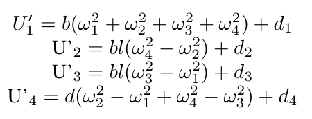
A quadrotor is considered an underactuated system as it has six degrees of freedom while only having four control inputs [3]-[4]. The four control inputs are U1- Thrust Force, U2 Roll Torque, U3- Pitch Torque, and U4- Yaw Torque.

where b,d are the lift and drag coefficients and l is the distance between the rotation of the axis of two opposite propellers. The rotational equations of motion are derived with respect to the body-fixed frame, while the linear motion equations are derived in the inertial frame. After a bit of transformation we end up with the nonlinear quadcopter model :

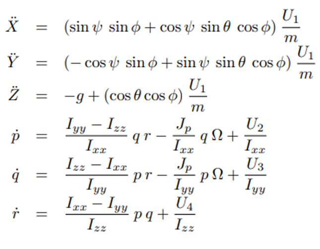
where Ixx, Iyy, Izz are the principal moment of inertia, Jp is the moment of inertia of the propeller ,p ,q ,r are the angular rates of the quadcopter,ϕ ,θ ,ψ are the roll, pitch and yaw angles and ω = ω2−ω1+ω4−ω3 .

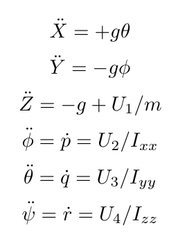
B. Linearized System Dynamics

Since we are attempting hover control, we linearize the dynamics about hovering conditions to get

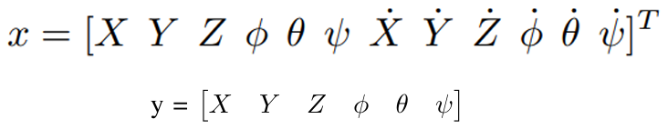
we choose our state x and observation y to be:

In the state space representation, we get

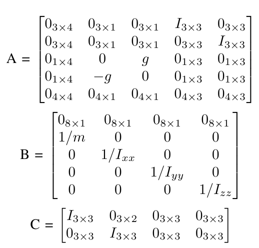
with D being a Null Matrix.

C. Exogenous Signals

The main objective, as stated earlier, is hover control even under uncertain conditions. The inputs U, U2, U3, U4 are the torques and thrust applied to the quadcopter. These forces are a function of parameters b and d, which are the aerodynamic force and moment constants, respectively. These values are determined experimentally. The sources of uncertainty could be from these two factors in addition to the values of m, I and l. The dynamics of the BLDC motor are not considered during the modelling, which could be another source of uncertainty. The observations for the system can be obtained relatively easily with a GPS and an IMU module.

The exogenous signals w consists of the disturbance d, the noise n and the reference signal r. The disturbance d, which could be caused by external gusts or winds, enters the system through the modified torque equations below

The noise n enters the system as a result of the sensors (i.e IMU and GPS module) we plan on using on the quadcopter. In addition, we also have the reference signal r entering the system here. This essentially means, Y = Cx + n+ r where

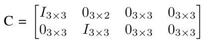
and Y is the output used by the controller as per the convention used in class.

Optimal Controller Formulation :

With the overall system linearized and with the exogenous signals identified, we will now set up the generalized plant and design a H-∞ controller.

A. Generalized Plant

As defined earlier, my exogenous signal w is defined by

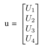
where r = [0]. My input signal u are the input torques defined by

And finally, the performance matrix z is defined by

where e = r − yp but as r = [0] we have e = −Yp and u = yc. A block diagram of the generalized plant is given in Fig 1.

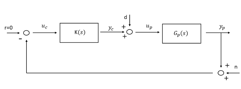
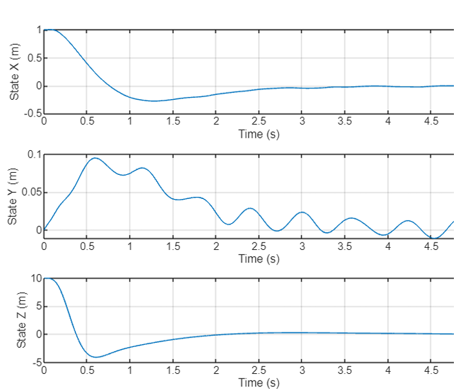
The exogeneous signal and performance were set depending on the environment conditions and instrument properties. Please look at the final report for a more details on the weights . With the chosen weights a H∞ norm of 0.77 for the controller was achieved. Fig. 2 and Fig. 3 plots the state response of the closed loop system.

Fig. 2 State X, Y, and Z Closed loop response with the synthesized H∞ controller

Fig.3 Roll, Pitch and Yaw Closed loop response with the synthesized H∞ controller

Uncertainty Modelling :

The are multiple parameters which are uncertain in the system. As mentioned earlier the control inputs are the torques U1,U2,U3,U4, which are a function of the angular velocity ω1,ω2, ω3, ω4 and the lift and drag coefficients b, d. The change in air density due to altitude, temperature and gusts can cause variations in these parameters. However, I feel that these variations could be captured by making the mass and inertia as uncertain parameters. Most literatures assume the quadcopter to carry a payload of an uncertain mass. [10] indicates that the proposed robust controller can effectively handle payload uncertainties up to at least 20 per cent. I will follow a slightly conservative change as I am not expecting the quadcopter to carry any payloads and assume the mass to have an uncertainty of 10 per cent.

Finding the changes in Inertia is more complicated as there are multiple factors to consider. While some articles suggest we could assume the inertia to increase proportionally to the changes in mass, I found no mathematical backing to this claim. I was also not able to find any work where I could find an upper bound to these changes. So, I am going to consider a change of 5 per cent in Inertia for all three axes. I am assuming the maximum change of 10 per cent in Mass would be sort of spread around all three axes, so it would be less than 10 per cent. I am also assuming the changes are mainly in the body of the quadcopter. Having an uncertain mass towards the extremes could cause the inertia to change at a higher percentage, but I will not consider these extreme cases. The sigma plot for the uncertain system can be found in Fig. 4 .

Fig. 5 Sigma Plot of the Uncertainty weight bound using ’ucover’

Robust Controller Formulation and Simulation :

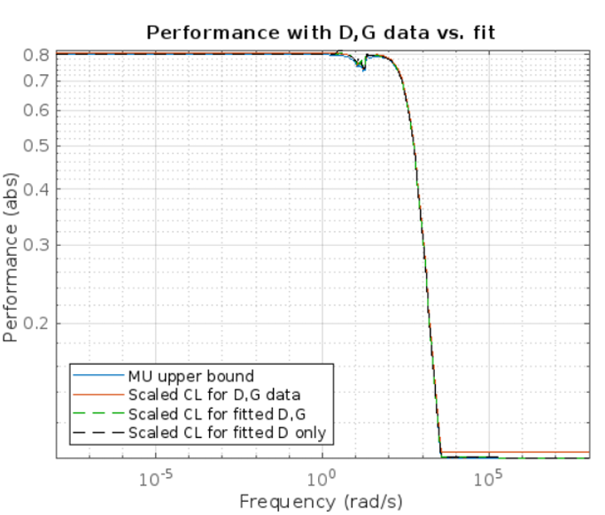
I used the DK iteration to generate a robust controller for the quadcopter in the presence of the model uncertainties as mentioned in the previous section. Since the system had 4 real uncertain parameters the musyn’s MixedMu option was set to ’on’ to allow the use of both the D-scaling and G-scaling. I have not restricted the maximum order of the scaling and used the default value. The maximum iteration was set to 20 although the iterations seemed to converge consistently within 5 iterations.

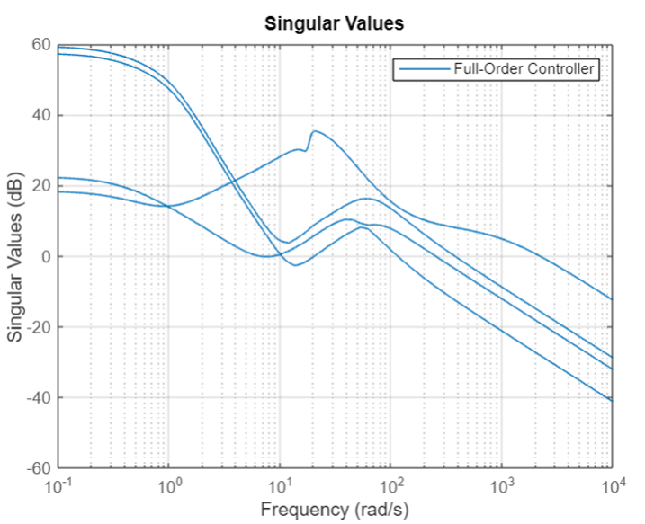
Although the order of my controller was 100, I have not reduced the order of the controller. In addition, the plots related to the controllers and the closed loop system response are all associated with a full order controller. The sigma plot for the synthesized controller is provided in figure 6 and the µ- plot is provided in figure 7. It can be seen that the worst case µ is approximately 0.8 which guarantees that the robustness condition is met.

Fig. 6: Sigma Plot of the robust controller designed using DGK iteration

Fig. 7: µ- plot of the robust controller designed using DGK-iteration

A. Closed-Loop simulation with Robust Controller and Nominal System Model:

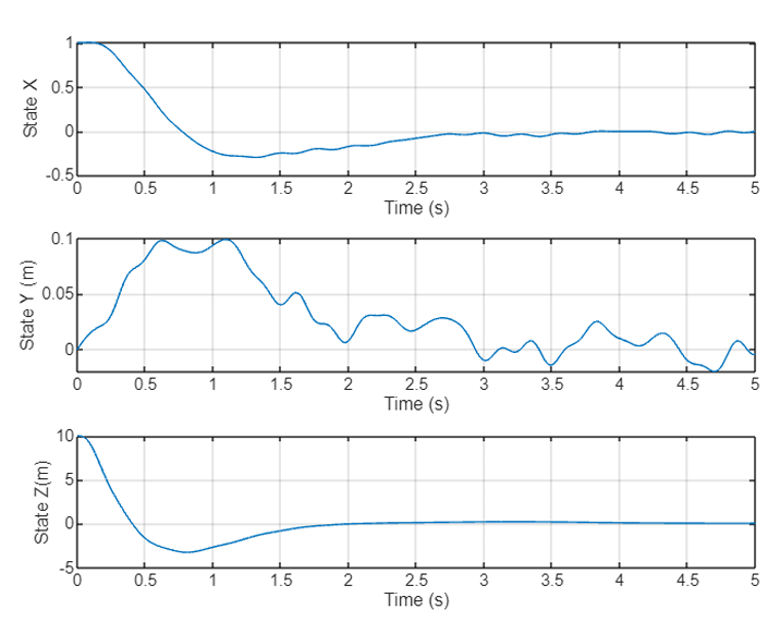
The robust controller synthesized using DGK-iteration was implemented in a simulation on the nominal linear model of the system. Fig 8. and 9 plots the system's response using the robust controller.

Fig. 8: State X, Y and Z Closed loop response with the synthesized robust controller

Fig. 9: Roll, Pitch and Yaw Closed loop response with the synthesized robust controller

B. Closed-Loop simulation with Robust Controller and Uncertain System Model:

The same robust controller was simulated with an uncertain linearized plant. Figure 10 and 11 has the system response sampled for 20 sampled plants. We can see that the response of the system is very reasonable and is well within our performance expectations.

Fig. 10: State X, Y, and Z Closed loop response with the sampled Uncertain plants

Fig. 10: Roll, Pitch and Yaw Closed loop response with the sampled Uncertain plants

The results of the simulations were discussed and found to be within performance expectations. This provides us with a useful and a practical controller which can be deployed on a quadcopter that can hover stably under wind disturbances. Future work on this topic could involve a more realistic sources of uncertainty such as combination of both parametric and dynamic uncertainty. In addition, the simulations were performed on only the linear system. Simulations on the Non linear model can provide us with more accurate results.

References:

[1] Kaufmann, E., Bauersfeld, L., Loquercio, A., M¨ uller, M., Koltun, V., Scaramuzza, D. (2023). Champion-level drone racing us ing deep reinforcement learning. Nature, 620(7976), 982–987. https://doi.org/10.1038/s41586-023-06419-4

[2] Panerati, Jacopo, et al. ”Learning to fly—a gym environment with pybullet physics for reinforcement learning of multi-agent quadcopter control.” 2021 IEEE/RSJ International Conference on Intelligent Robots and Systems (IROS). IEEE, 2021.

[3] IEEE Systems, M., Institute of Electrical and Electronics Engineers. (n.d.). Conference proceedings: 2016 International Conference on Ad vanced Mechatronic Systems: Nov. 30- Dec. 3, 2016, Melbourne, Australia.

[4] Araar, O., Aouf, N. (n.d.). Full Linear Control of a Quadrotor UAV, LQ vs H .

[5] Tahir, Z., Jamil, M., Ali Liaqat, S., Omer Gilani, S., Tahir Waleed Tahir Saad Ali Liaqat, Z. (2016). State Space System Modeling of a Quad Copter UAV State Space System Modelling of a Quad Copter UAV. Article in Indian Journal of Science and Technology. https://doi.org/10.48550/arXiv.1908.07401

[6] Oktay, T. Kose, O.. (2019). Dynamic Modeling and Simulation of Quadrotor for Different Flight Conditions. European Journal of Science and Technology, (15), 132-142. [7] Asignacion, A., Suzuki, S., Noda, R., Nakata, T., Liu, H. (2022). Frequency-Based Wind Gust Estimation for Quadrotors Using a Nonlin ear Disturbance Observer. IEEE Robotics and Automation Letters, 7(4), 9224–9231. https://doi.org/10.1109/LRA.2022.3190073

[8] Hattenberger, G., Bronz, M., Condomines, J. P. (2023). Evaluation of drag coefficient for a quadrotor model. International Journal of Micro Air Vehicles

[9] https://invensense.tdk.com/wp-content/uploads/2015/02/PS-MPU 9250A-01-v1.1.pdf [10] Dhadekar, D.D., Sanghani, P.D., Mangrulkar, K.K. et al. Robust Control of Quadrotor using Uncertainty and Disturbance Estimation. J Intell Robot Syst 101, 60 (2021). https://doi.org/10.1007/s10846-021-01325-1